Statistics is a discipline that develops and applies scientific methods in collecting, analyzing and interpreting data. These scientific methods that are frequently applied include designing and analyzing surveys and experiments, quantifying of the social, scientific and biological phenomenon and statistical principles application in understanding the world around us. Therefore, statistics is a wide area of study that can be applied in medical, biological, research institutes, government, management, manufacturing, marketing research, finance, economics and social sciences (Abelson, 1995, p.44).
T-test or the students’ t-test is a statistical concept that was developed by William Gosset in 1908. He developed it in efforts of making sure that each batch of Guinness he manufactured was as similar as possible to the other. It is thus used to compare two groups. T-test is the most widely known and used the statistical test. This is because it is straightforward, simple, adaptable to broad range situations and easy to use. The utility of this method is occasioned by the fact that many scientific researchers are out to examine relatedness phenomenon involving two elements at a particular time. In t-tests, the big interest rests on the comparison of the two means. It is best expressed by spelling out the difference in means of a data that may involve effect size, percent difference or raw units. The critical consideration is given to the magnitudes of both the difference and confidence limits (Kimble, 1998, p.67).
The t-test is a test which after performing the statistical hypothesis test, the test statistic shows a student’s t distribution and the null hypothesis tied to this analysis is true. It is mostly applied in a case where sample sizes are small and normally distributed. The statistic of inference is not normally distributed for it does not rely on precisely known value but on uncertain estimated standard deviation. One of the uses of t-test is confirming whether a mean of a population that is normally distributed is a value within the specification of the null hypothesis. It is also used to test a hypothesis that states means of two populations that are normally distributed are equal. These populations have different data sets, with a different number of data points, standard deviation, and means. In the calculation of this statistic, it is assumed that population distributions are normal, variances are equal and samples are either dependent or independent (Abelson, 1995, p.45).
Student’s t-test can either be paired or unpaired. Paired t-test is a criterion applied when data points of both groups in consideration correspond. The unpaired t-test is used regardless of whether or not the two groups have correspondence in data points. This may be a case where variances or means could differ. The advantage of paired t-test method is that the procedure used is simple.
It starts with a null hypothesis that the means of both groups are equal, an assumption that can only be proved by considering the variances. A value to represent the significance level is set, probably α = 0.05 or 5%. The differences for each pair are calculated, which should be measured at the same time. A histogram of these differences is plotted to determine whether they are normally distributed. Means and standard deviations of both sets of differences are calculated.
The value of t is then calculated using the following formula;

Where; dav is the mean of the differences calculated from the pairs. SD is the standard deviation of the two differences. N is the number of pairs that have been put into consideration. T is the t value to be interpreted, of which the sign whether positive or negative does not matter (Kimble, 1998, p.68).
The significance level (α) is looked up where it lies in attachment with the t value that has been obtained. This check is performed by appropriate software of the table of t distribution. For this to be accomplished, it is vital to determine the degrees of freedom. For this test, the degrees of freedom are obtained by taking the number of pairs less one (n-1). At this stage, it is necessary to find out whether the analysis concerns one tailed or two tailed tests. This is because we can not be fully sure that we have to accept or reject the null hypothesis. If a true null hypothesis is rejected, a type 1 error is committed. Failure to reject a false null hypothesis is committing of type 11 error. It is statistically preferred to commit type 11 error compared to type 1 error for the sake of conserving accuracy of the t statistic. If the critical value of t is less than the calculated value, the null hypothesis is rejected, evidencing significant statistical difference between the groups. If the critical value is greater than the calculated, the null hypothesis is accepted, because there exists no statistical support of any difference between the two groups.
For a case of unpaired test, the following formula is used.
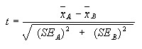 , where;
 refers to means of the two groups, SE refers to standard deviations of the two groups. The degrees of freedom, in this case, are obtained by adding the number of values in the two groups less two. Interpretation of the t statistic is similar to the one of paired test (Abelson, 1995, p.45).
Reference:
- Abelson Robert, 1995. Statistics as Principled Argument in Analysis. Lawrence Erlbaum Associates, London, pp. 44, 45.
- Kimble Gregory, 1998. How to Use and Misuse t-test in Statistics. Prentice Hall Press, New York, pp.67, 78.